Working Results
Relevant zip files full of information have been moved to make way for the question and answer
section below. Check here if you're looking for a specific file that
you don't have the address to.
Questions and Answers
In many respects, the main questions motivating much of our work has
been What determines the saturation of speed-up with
the number of processors? Thus far all of our work has been
focused on strong scalability (fixed problem size but increasing
processors), but that isn't a necessity for everything we're interested
in.
The follow-up question to the saturation limits is whether or not we can
overcome these initial issues. Hopefully below we address as much of
this as is possible and provide numerical evidence to support our
conclusions.
Note that the most significant of these results were presented at the
APS-DPP meeting in November. When appropriate I'll not that the results
were presented there. Also as we continue to present more stuff that
material will also be posted here. Upcoming stuff includes the FACETS
meeting in February and SIAM-CSE11.
LOGOS I've used some very high resolution pictures for presentations and posters in the past. Those can be found
here.
Considering a 1D radial decomposition
Our initial experiments starting back in Fall 2009 and continuing until
Spring 2010 dealt with the use of the LU decomposition as the primary
solver for UEDGE. Because of the desire to conduct simulations with
active neutral gas terms our initial belief was that the direct solver
was needed for the linear solves.
In fact, that belief may be valid for some steady state simulations.
Recall that we use a very large time step (dt = O(1)) to incur a steady state simulation.
Thus knowledge of the effect of the time step is significant in determining an acceptable solver.
Question: What effect does the choice of time step have on the 1D decomposition?
Answer: Decreasing the time step increases the validity of ASM.
That's the one line answer, but the picture is more complicated than that if we consider more than just the time
step as variable.
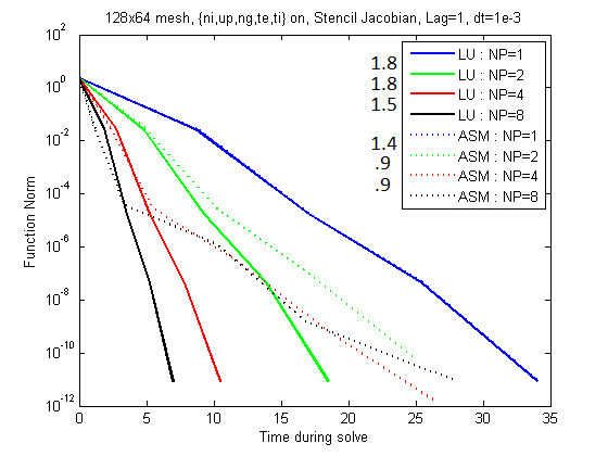
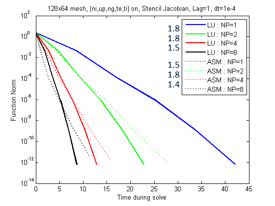
Below there are pictures showing the deteriorating scalability for increasing time steps with the neutral
equations active.
Note that these images were generated using Jacobian lag=1.
Figure 1: Note the speed-up values listed to the left of the legend.
The images above indicate that the scalability of the LU decomposition
is unaffected by dt, although it does suffer its traditional limitations.
The ASM preconditioner does falter significantly for larger time steps
and actually fails to converge for sufficiently high number of
processors with large enough time steps. This is part of what confirmed
our belief that the direct solver is necessary when incorporating
neutral gases for steady state simulations.
For small enough time steps we can have a different solver than LU and still solve the system.
Of course, we're not just interested in solving the system at all, but eventually solving it as quickly as
possible.
To try and answer that we need to understand what effect the component equations are having on the solver.
The common belief is that the neutral gas terms are holding back the performance, which leads to the following.
Question: What effect does the choice of time step have on the 1D decomposition in
the absense of neutrals? (plasma equations only)
Answers: For smaller time steps, ASM is the optimum solver.
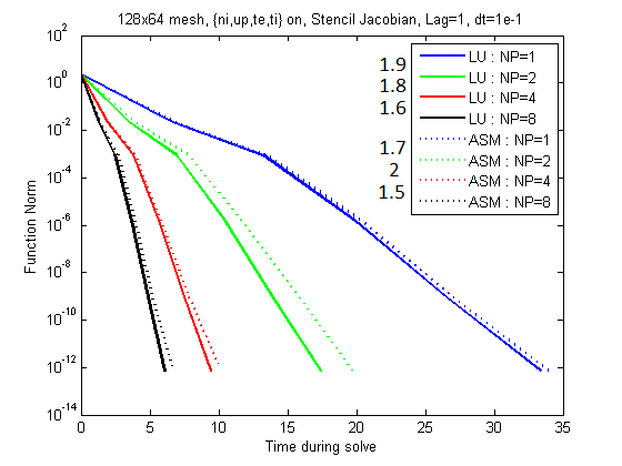
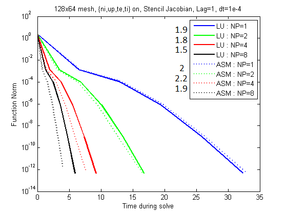
Below are graphs that show the effect of the time step on the plasma equations only.
Figure 2: Note the speed-up values listed to the left of the legend.
Once again we see the improvement in speed for ASM and the time step agnosticism for LU.
The surprising feature here is that the gain in scalability with ASM eventually overcomes the loss in quality due
to neglected coupling between domains.
This in my mind helps confirm our belief that the presence of the neutrals is what causes the loss of
scalability in ASM.
The next test which is logical to help supplement our scalability concerns is to analyze the solver in the absense
of plasma equations - with neutral terms only.
Question: What effect does the choice of time step have on the 1D decomposition in
the absense of plasma equations? (neutral terms only)
Answers: Tests underway (Assumed to have AMG preferred no matter what)
I expect that when these tests are done we will see multigrid as the preferred solver, but there is no guarantee
that the difference between multigrid and LU will be significant.
There's obviously a lot of tuning parameters for mutligrid, so there may be something to look at there.
For the time being, let's work under the assumption that AMG is optimal and I'll fix that if the experiments come
back otherwise.
Thus far I have been using the term ASM without appropriately defining it.
ASM is the Additive Schwarz domain decomposition based solver with overlap=1 and LU solver on each domain.
The term overlap roughly refers to how much coupling between disjoint domains is allowed.
Each domain has its own solver, although they are always the same type of solver.
Given this information about ASM, it is reasonable to ask whether these overlap=1 and LU sub_solver defaults are
appropriate. Let's examine that below.
Question: What effect does the amount of overlap have on the ASM solver assuming
dt=1e-4?
Answer: Increasing the overlap improves the total speed of the solve, to a point.
What we see in the picture below is that there is a significant difference between overlap=0 and overlap=1.
Note that the overlap=0 case is the block Jacobi style of domain decomposition, and increasing the overlap pushes
the solver towards the fully coupled solution.
Recall that the bars are scaled so that all the bars will be of equal height in the event of optimal
strong scalability (n times additional processors runs in 1/n as much time).
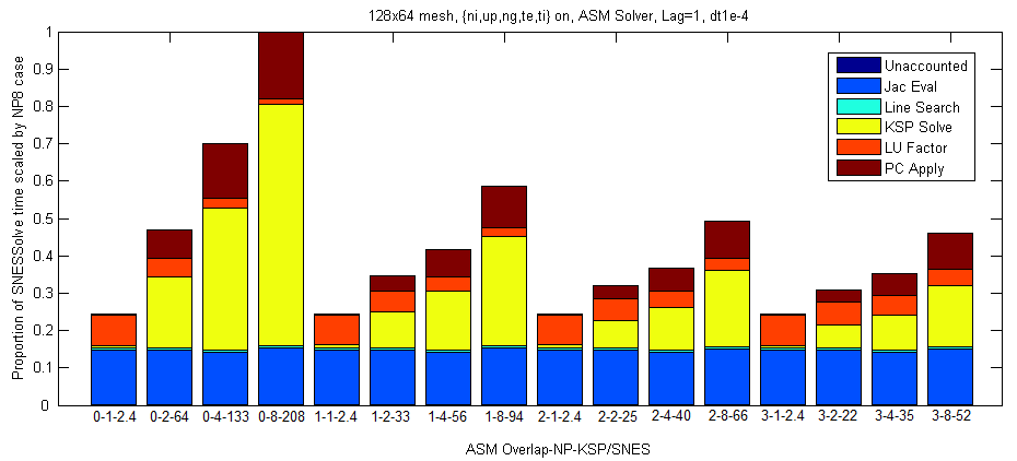
Figure 3: Note the average linear iterations per nonlinear iteration listed beneath each experiment.
Of significance here is the great improvement in scalability initially which tapers off as the overlap increases.
Also note the shift in computational time from KSP Solve and PC Apply to LU Factor.
This is because the quality of the preconditioner is improving with increasing overlap and thus fewer linear
iterations are required.
The cost of that better preconditioner is that more work is required to create it.
Question: What effect does the choice of sub_solver have on the 1D decomposition
assuming dt=1e-4?
Answers: No significant difference ... for NP≤8
This result is only partially complete because of the difficulties we've had in running on more than 8 processors.
So far it seems like LU or ILU are both equally fine, for the time step we've chosen.
It does look like for larger NP we would see benefits in using ILU, but I'd have to do an experiment to confirm.
It would also be valuable to consider the effect for other time steps.
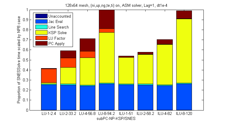
Figure 4: Note the average linear iterations per nonlinear iteration listed beneath each experiment.
For the moment, it seems as though the standard choices for Additive Schwarz are appropriate, although as the
conditions of our experiments change we may need to evaluate.
One big change that should be introduced now is the use of a physics preconditioner which we refer to in the PETSc
terminology as FieldSplit.
Here the terms "physics preconditioner", "component-wise preconditioner", "operator-specific preconditioner" are
all used interchangeably.
Question: Assuming dt=1e-4, how can we use what we've learned so far to
produce a better solver?
Answers: FieldSplit preconditioner using the optimal solvers on subsets of the
variables.
The structure of the physics preconditioner used here, as well as a broader discussion of existing and potential
FieldSplit options will be provided elsewhere.
For the time being, this solver consists of two blocks where the plasma terms are solved independently of the
neutral terms and vice versa.
Any coupling between the two terms is neglected for simplicity, but may be of significance in future experiments.
Each set of variables is solved with its optimal solver: neutrals - AMG; plasma - ASM.
The scalability results can be seen below.
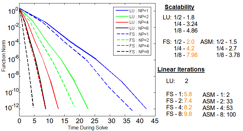
Figure 5: Relevant information showing the effectiveness of FieldSplit over LU given to the right.
Even with this simple splitting of the problem, the significance of operator-specific preconditioning is
immediately obvious.
The strong scalability of the solver is near optimal for up to 8 processors, and the number of linear iterations
doesn't undergo the explosion that we see for ASM.
This allows for the FieldSplit preconditioner to outperform LU not just in scalability, but in total time as well.
There are some questions that can be raised with FieldSplit given these results.
Question: What effect does the time step have on the effectiveness of FieldSplit?
Answers: Tests underway (Assumed tendency toward LU speed)
Experiments will need to be done to determine the usefulness of FieldSplit for larger time steps, although my guess
is that there will be solid performance even for larger time steps.
I feel that way because the ASM on plasma only at dt=1e-1 was about equivalent to LU, so I doubt FS would do
any worse than LU.
Given that I imagine that for appropriately large time steps the FS preconditioner will behave much like the LU
preconditioner as that will begin to dominate the computation.
Another issue we haven't tackled so far is the Jacobian lag.
We don't want to have to reevaluate the Jacobian at each SNES step if the previous Jacobian is still a "good
enough" preconditioner.
If FieldSplit is going to be the preferred 1D solver, we need to determine its usefulness for other lags.
Question: What effect does the Jacobian lag have on the effectiveness of FieldSplit?
Answers: Lag up to 5 has no detrimental effect on FieldSplit
The experiments above all have Jacobian lag equal to 1 as the default, but for a production level code we would
want to have the solver work with higher lag values.
The graph below compares the speed of the solve for LU and FS given lag=5.
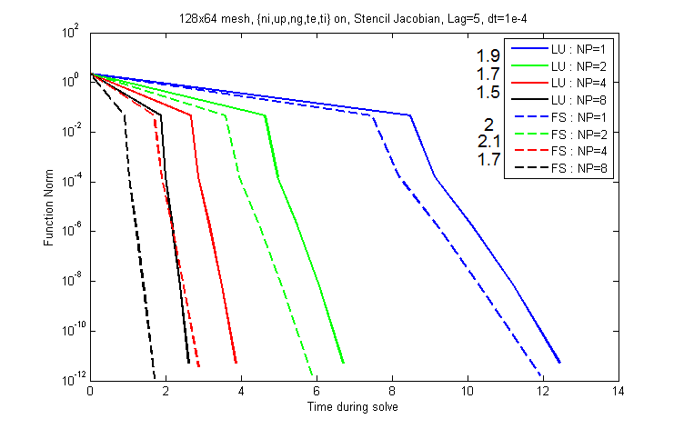
Figure 5: Scalability information is listed to the left of the legend.
Here we see roughly the same level of outperformance of FS over LU.
This is somewhat surprising because it was previously assumed that without a low lag the solver would take too many
linear iterations and lose its edge.
Instead we see that is not the case, although the same can't necessarily be said for larger time steps, or even in
the multistepping case.
We'll need more experiments to say something about that.