425/525 Statistical Methods
Spring 2010
Instructor: Michael McCourt
SPSS References: Conducting Independent Samples t Tests
Note that this section is rather long. In case you're looking for some small piece of info, I've anchored a few items that you may find useful:
For this tutorials let's take a look at the Systolic Blood Pressure data set in the SPSS main page. In fact, to make things simpler, let's only look at the math stress columns and the Sex identifier. If we delete all columns except those we are left with just the data below.
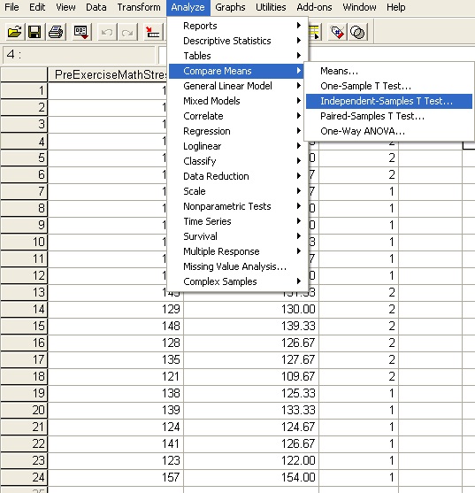
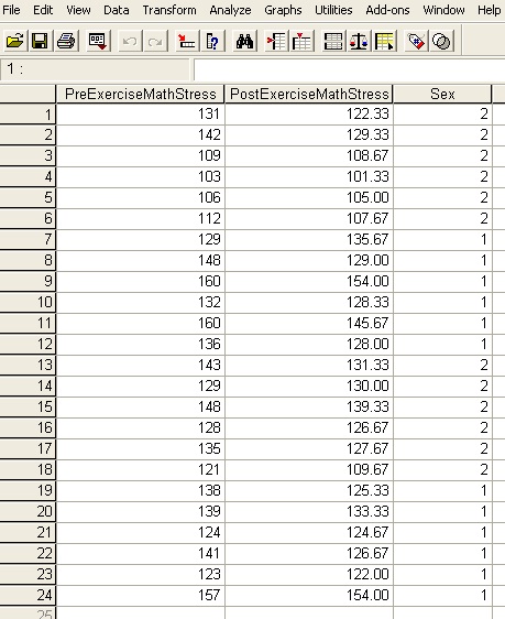 If you were asked to test the data set PreExerciseMathStress to see if the mean of the distribution that generated it was 135, you would want to run a one-sample t test. If instead we are interested in comparing the difference between how men and women responded to Pre-Exercise Math Stress, we would want to run an independent samples t test. To do so, we click Analyze>Compare Means>Independent Samples t Test to open the necessary dialog.
 Once in the dialog, the data you are interested in studying needs to get moved to the Test Variable(s) box, in this case Pre-Exercise Math Stress. You also need to supply SPSS with the means to differentiate between males and females. To do this we need to move the Sex column over to the Grouping Variable box.
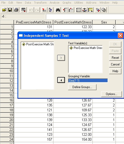 Even though we have told SPSS that we are grouping the input data by Sex, we have to still tell it what the two groups we are interested in studying are. This is important in case the data provided were categorical rather than numerical, or if there were more than two groups since we would only be able to study two at a time. To tell SPSS how to identify the two groups we want to study, we click the Define Groups option under the Grouping Variable box.
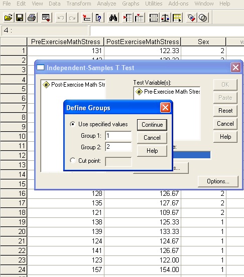 Now we have a new dialog to consider. Since we identify the groups by Male=1 and Female=2, we tell SPSS that 1 and 2 are the values of the groups we are interested in. Likewise if the column had values of Male=M and Female=F we would tell SPSS that M and F are the values of the groups. If there were values Black=1, Brown=2, Blonde=3 and we were interested in a t test between Black and Blond, you would give SPSS the values 1 and 3. Once the necessary groups are identified, click Continue and then OK to see the results of the test.
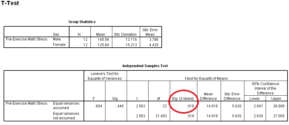 Feel free to ignore the "Equal variances not assumed" column as we never talked about this in class (although the material is mentioned in the later parts of chapter 10). Looking strictly at "Equal variances assumed" we see that the significance value is less than α=.05 which means we can reject our null hypothesis and conclude that men and women do not have the same Pre-Exercise Math Stress.
As was talked about in the One-Sample section, you may feel free to run multiple tests simultaneously by moving more than one column into the Test Variable(s) box. The only other thing worth mentioning here would be the use of the cut-point option to group data with. Suppose we were interested in seeing what effect having a Pre-Exercise Math Stress of greater than 133 had on your Post-Exercise Math Stress. There are two ways to do this: Create a new column of data which describes these groups (≥133 or <133) or use the cut point option in the Define Groups dialog.
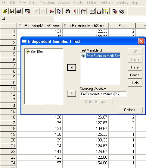
Let's look first at the cut point option since this is part of the t test concept. Here we move Post-Exercise Math Stress into the Test Variable(s) box, but rather than grouping by Sex, we want to group by Pre-Exercise Math Stress value. This looks like the following.
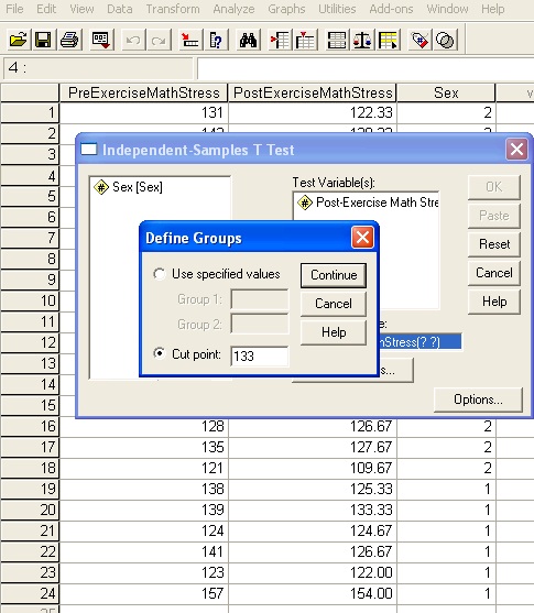
 Now when we enter the Define Groups dialog, instead of choosing the "Use Specified Values" option, you're going to use the "Cut Point" option. Select that radio button and then enter the value of 133, since we want to study people who had Pre-Exercise stress above 133 and below 133.
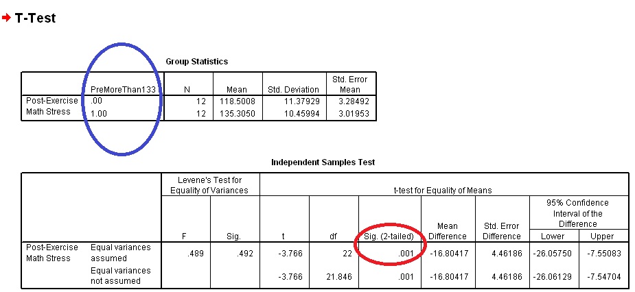
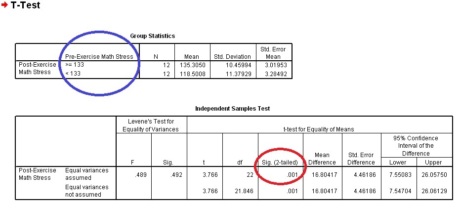
 After we click Continue and OK, we can review the results of the test. Notice the Blue circle highlighting the classification we are making by using the Cut Point option. Also, as always, note the result of the test circled in Red. Since this value is less than α=.05 we can reject the null hypothesis that people who had high Pre-Exercise Math Stress and people who had low Pre-Exercise Math Stress had the same Post-Exercise Math Stress.
 I said there were two ways of handling this two-sample t test. The other way is to create a new column of variables for which people with Pre-Exercise Math Stress ≥133 have a value 0 and people with Pre-Exercise Math Stress <133 have value 1. To do this, open the Transform>Compute tab as shown below.
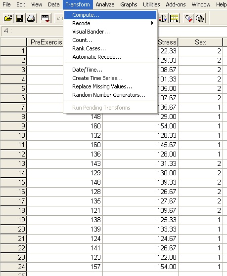 This will open a dialog that may look very intimidating - we're going to break it down into steps. First you need to name your new classifying column. Choose a name that makes sense to you: I chose PreMoreThan133. Put that name into the Target Variable box which in the picture below is circled in red.
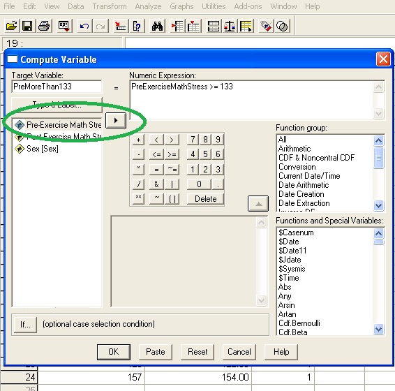
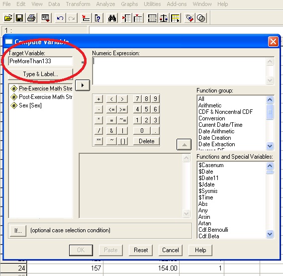 Now, in numeric expression we need to come up with an expression that would give a value 0 for pre-stress≥133 and a value 1 for post-stress<133. To do this we exploit the fact that in computer science logical expressions evaluate to 1 for true and 0 for false. As a result when we the computer sees the expression (PreExerciseMathStress≥133) that takes value 0 for false and 1 for true. Try putting that statement into the Numeric Expression box. Note that you need to click on the Pre-Exercise Math Stress object in the box on the left and move it to the Numeric Expression box using the arrow button (circled in green in the image below).
 If everything is entered correctly, after we push OK we should see our new column appear below. Note that you can feel free to change the number of decimal places that show up in the "Variable View" tab on the bottom of the spreadsheet.
 At this point you can just conduct a normal independent-samples t test with the Grouping Variable PreMoreThan133. If you've done that correctly you should see the output below. Notice how it is almost identical to the results from using the Cut Point method (as it should be) with the exception of the material inside the blue circle.