SplineDemo.m
Contents
Overview
Illustrates cubic spline interpolation by calling MATLAB's built-in spline function (for not-a-knot splines and clamped splines) and a modified version of splinetx (from NCM) (for natural splines). The functions evaluate the cubic spline interpolating the data specified in the vectors x and y at all of the points in the vector u.
As output we get plots of
- the data,
- and a smooth MATLAB graph.
Initialization
clear all
close all
% Define the data and evaluation points
x = [0 1 3 5 6];
y = [2 -3 1 2 4];
u = linspace(0,6,100);
Call splinetx_natural
Evaluate cubic natural spline interpolant at u
v = splinetx_natural(x,y,u);
Plots
Plot the data
hold on
xlim([-1 7])
ylim([-4 5])
title('Cubic Natural Spline Interpolant')
plot(x,y,'bo','LineWidth',2)
legend('Data','Location','NorthWest')
pause

Use MATLAB to get a continuous graph
plot(u,v,'r','LineWidth',2)
legend('Data','MATLAB graph','Location','NorthWest')
hold off
pause

Call spline
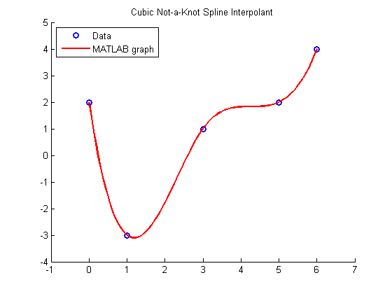
Evaluate cubic not-a-knot spline interpolant at u We could also use splinetx here.
v = spline(x,y,u);
Plots
Plot the data
figure
hold on
xlim([-1 7])
ylim([-4 5])
title('Cubic Not-a-Knot Spline Interpolant')
plot(x,y,'bo','LineWidth',2)
legend('Data','Location','NorthWest')
pause

Use MATLAB to get a continuous graph
plot(u,v,'r','LineWidth',2)
legend('Data','MATLAB graph','Location','NorthWest')
hold off
pause
Call spline again
Repeat with cubic clamped spline defined in spline y(1) and y(end) contain the values of the slopes at left and right endpoints
y = [10 y -10];
% Evaluate cubic clamped spline interpolant at u
v = spline(x,y,u);
Plots
Plot the data
figure
hold on
xlim([-1 7])
ylim([-4 5])
title('Cubic Clamped Spline Interpolant')
plot(x,y(2:end-1),'bo','LineWidth',2)
legend('Data','Location','NorthWest')
pause

Use MATLAB to get a continuous graph
plot(u,v,'r','LineWidth',2)
legend('Data','MATLAB graph','Location','NorthWest')
hold off
